The Gist of Algebraic Geometry
Contents
1. Intended Audience
The imagined audience for this post is someone with some non-math STEM training, maybe in physics or computer science, who either:
- Is interested in applications of algebraic geometry to their field, or
- Is my friend, and wants to know about my academic research.
We’re not going very in depth here. The goal is to give a taste of algebraic geometry so you can decide if you want to know more, or to act as a primer for more detailed material.
I’ll be assuming that you know what polynomials are, and that you’re comfortable with basic math symbols and notation (like $\mathbb{R}$, $\in$,$\subset$) at the level of a first-year university algebra or discrete math course. I will not be assuming that you know what rings and ideals are, but if you do, then you should have no problem following along.
2. Algebra
To start us on the same page, let’s review the algebra of polynomials. Given a set of numbers (a ring) $k$, we let $k[x]$ denote single-variable polynomials whose coefficients are in $k$. For example, $\mathbb{Z}[x]$ contains elements like $4x^3 - 2x + 1$, and $\mathbb{R}[x]$ contains elements like $\sqrt{2}x^2 + 0.3x - \pi$. Of course, since the integers are contained in the real numbers, we have $\mathbb{Z}[x] \subset \mathbb{R}[x]$. We don’t need to restrict ourselves to a single variable either: we let $k[x_1,x_2,…,x_n]$ denote polynomials with multiple variables. For example $\mathbb{Z}[x,y]$ contains elements like $3x^2y - x^2 + 9xy + y$.
These polynomial rings have addition and multiplication operations, by adding and multiplying polynomials just as you learned in highschool. For example,
\[(x^2+3)\cdot(x^3 + 2x + 1) = x^5 + 5x^3 + x^2 +6x + 3.\]Importantly, given two polynomials $f$ and $g$ inside $k[x_1,…,x_n]$, we can ask if $f$ divides $g$. Given two integers $a,b\in\mathbb{Z}$, we say that $a$ divides $b$ if there exists another integer $k$ such that $b = a\cdot k$. So, for two polynomials $f$ and $g$ inside $k[x_1,…,x_n]$ we will also say that $f$ divides $g$ if there exists another polynomial $h$ such that $g = f\cdot h$.
For example, does $f(x) = x^2 + 1$ divide $g(x) = x^3+3x^2+x+3$? Yes, because $g(x) = (x+3)\cdot f(x)$.
To find the polynomial $h$ such that $g = hf$, you can use polynomial long division! You probably learned how to do this in highschool for single-variable polynomials, but if you’re like me, you’ve long since forgotten. Maybe this is a good chance to review it, and try confirming that $(x^3+3x^2+x+3) / (x^2 + 1) = x+3$!
Inside of these polynomial rings, we are interested in special types of sets which let us generalize the idea of modular arithmetic. Before we define them, let’s review modular arithmetic. Pick any integer $m \in \mathbb{Z}$. We say the integers mod $m$ are what you get by declaring that everything which is divisible by $m$ is now equal to $0$.
For example, take $m=24$. Then we are declaring that $24\equiv 0$, $48\equiv 0$, and so on. What about, say, 32? Well, $32=24+8$ and $24\equiv 0$, therefore $32 \equiv 8$, modulo 24. If you’ve done some programming, you may recognize this as as the modulo operator; 32 % 24 will return 8 in most languages. This is also how clocks work – if it is 1pm, and I tell you that something will happen in 32 hours, you mentally compute that $32 \equiv 8$ and then know that the event will occur at 9pm the next day. Formally, one defines $\langle m \rangle$ to be the set of all integers that are divisible by $m$. Then, we use the notation $\mathbb{Z}/\langle m \rangle$ to mean the integers modulo $m$.
Now let’s return to polynomials. Given any polynomial $f \in k[x_1,…,x_n]$, we can define $\langle f \rangle$ to be the set of all polynomials in $k[x_1,…,x_n]$ which are divisible by $f$. This is called the ideal generated by $f$. Then, we can let $k[x_1,…,x_n]/\langle f\rangle$ be the set of polynomials modulo $f$, by setting everything in $\langle f \rangle$ equal to $0$.
Setting everything in $\langle f \rangle$ equal to $0$ is the same as setting $f=0$. This is because $g\in\langle f\rangle$ means that $f$ divides $g$ so $g = fh$ for some other polynomial $h$. Then if we set $f=0$, we get $g=0h=0$!
Example: Consider $x^2 \in \mathbb{R}[x,y]$. What polynomials are in $\langle x^2 \rangle$? Well, if $g \in \langle x^2 \rangle$, then it must be divisble by $x^2$, meaning that there exists some polynomial $h$ such that $g = x^2 h$. For example, $g(x) = x^2(xy+1)$ and $g(x) = x^2y$ are in $\langle x^2\rangle$, but $g(x) = x+1$ is not.
Now, we can consider $\mathbb{R}[x,y]/\langle x^2\rangle$. A general polynomial in $\mathbb{R}[x,y]$ can be written as
\[f(x,y) = \sum_{i=0}^\infty \sum_{j=0}^\infty c_{ij} x^i y^j = c_{00} + c_{10}x + c_{01} y + c_{11}xy + \cdots\]However in $\mathbb{R}[x,y]/\langle x^2\rangle$ we are setting $x^2\equiv 0$. This also means $x^3 \equiv 0$, since $x^3 = x\cdot x^2$, and similarly $x^i \equiv 0$ for any $i\geq 2$. Therefore, all the terms in $f(x,y)$ that have $x^i$ in them, for $i\geq 0$ are now equivalent to 0. So we get
\[f(x,y) \text{ modulo } x^2 = \sum_{i=0}^1\sum_{j=0}^\infty c_{ij}x^iy^j = \sum_{j=0}^\infty c_{0j}y^j + x\left(\sum_{j=0}^\infty c_{1j}y^j\right).\]Informally, an ideal is a subset $I$ of $k[x_1,…,x_n]$ with the properties that ensure that doing modular arithmetic modulo $I$ is well-defined. We can compute $f$ modulo $I$ by setting everything in $I$ to $0$, and we denote the set of elements in $k[x_1,…,x_n]$ modulo $I$ as $k[x_1,…,x_n]/I$.
3. Geometry
Now let’s get to the pretty pictures part of math – geometry. One way to come up with curves on the 2D plane is to start with a function $f(x,y)$, and then plot all the points $(x,y) \in \mathbb{R}^2$ such that $f(x,y) =0$. For example, here is the curve whose points satisfy $y^2-x^3+x^2 = 0$.
Why specifically $f(x,y)=0$, and not something like $f(x,y) = 5$? Well, we could define a new functon $g(x,y) = f(x,y)-5$, and then $f(x,y)=5$ is equivalent to $g(x,y)=0$. This lets us simplify things a bit by always setting our function equal to $0$. When $f(x,y)$ is a polynomial, we call this set of points an algebraic curve, and it is the type of thing we can study with algebraic geometry.
We can get more than just curves in the plane. Given a polynomial $f \in \mathbb{R}[x_1,…,x_n]$, the points $(x_1,…,x_n)\in\mathbb{R}^n$ where $f(x_1,…,x_n)=0$ will define a hypersurface of dimension $n-1$ inside $\mathbb{R}^n$. We call this hypersurface the vanishing locus of $f$, denoted $V(f)$. This includes familiar shapes, such as the above saddle in 3D, given by the vanishing locus of $f(x_1,x_2,x_3) = x_3-2x_1^2+(y_2-1)^2$, and very unfamiliar shapes, such as these:
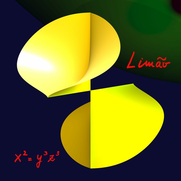
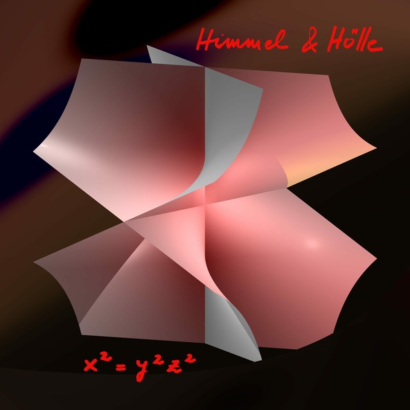
Notice how the defining equations of the Limão and Himmel & Hoelle are very similar, $x^2-y^3z^3$ and $x^2-y^2z^2$, yet the resulting surfaces are emphatically different!
It’s also possible to construct lower-dimensional shapes, like curves in 3D. This is done by taking multiple polynomials, and then looking at the set of points where they all vanish. This is the same as taking the intersection of their vanishing loci. For example, if $f(x,y,z) = x^2+y^2+z^2-1$, and $g(x,y,z) = \frac{1}{2}x-y$, then $V(f)$ is a sphere of radius 1, $V(g)$ is a plane through the origin, and their intersection is a 1D curve inside 3D, which is one of the great circles on $V(f)$.
In section 1, we defined the ideal generated by $f$, $\langle f \rangle$ inside $k[x_1,…,x_n]$, to be the set of $g\in k[x_1,…,x_n]$ such that $f$ divides $g$. We can extend this definition to multiple polynomials, and define $\langle f_1,…,f_k \rangle$, the ideal generated by $f_1,…,f_k$ to be the set of $g\in k[x_1,…,x_n]$ which are divisible by any of the $f_i$. For any ideal $I$ in $k[x_1,…,x_n]$, we define the vanishing locus $V(I)$ of the ideal to be the set of points in $k^n$ which are zeros of all the polynomials in $I$. These vanishing loci are examples of algebraic varieties, the main object of study in (classical) algebraic geometry.
4. Algebraic Geometry
The key idea in algebraic geometry is that the two stories we just discussed are really one and the same. In section 2, we saw that we can turn polynomials into geometric shapes, and it turns out that this process is reversable. That is to say, knowing the polynomial functions on a variety determines everything about the variety.
What do we mean by polynomial functions on a variety? Well, we know what the polynomial functions that take values in $\mathbb{R}^n$ are - we pick a co-ordinate basis $x_1,…,x_n$ for $\mathbb{R}^n$, and then the polynomials are $\mathbb{R}[x_1,…,x_n]$. Then for any subset $S$ of $\mathbb{R}^n$ we can restrict polynomials to $S$ to get polynomial functions on $S$.
However, many different polynomials are equal when you restrict them to a subset. Consider $f(x,y) = x$ in $\mathbb{R}[x,y]$, which defines $V(x)$ inside $\mathbb{R}^2$. $V(x)$ is the set of points where $x=0$, namely the $y$-axis. So the restriction of $g(x,y)$ to $V(x)$ is $g(0,y)$. This means the following functions are all equal on $V(x)$:
\[x+y, \quad x(y^2+3y+1)+y, \quad y(x+1)\]and many (infinitely) more.
This means that simply taking $\mathbb{R}[x_1,…,x_n]$ and restricting it to a variety grossly overcounts the number of true functions. Luckily, we learned how to deal with this in section 1! Two functions will be equal on $V(f)$, if they are equal modulo $f$.
Remember, taking a polynomial $g$ modulo $f$ means setting everything divisible by $f$ equal to 0. In our previous example, with $f(x,y) = x$, that means we get
\[x+y \equiv 0 +y = y,\] \[x(y^2+3y+1)+y \equiv 0(y^2+3y+1)+y = y,\] \[\quad y(x+1) \equiv y(0+1) = y.\]Thus, all of these functions are equal to $y$ modulo $x$. We say they are in the equivalence class of $y$. This tells us that the set of polynomial functions on $V(f)$, for $f\in k[x_1,…,x_n]$ is exactly $k[x_1,…,x_n]/\langle f \rangle$.
With this, we have our putative correspondance between algebraic varieties of $k^n$ and ideals $I$ inside the polynomial ring $k[x_1,…,x_n]$: we send the ideal $I=\langle f_1,…,f_n \rangle$ to the vanishing locus $V(I)$, and we send a variety $V$ to its ring of polynomial functions. However, there is one1 outstanding issue…
Consider the polynomials $x$ and $x^2$ in $\mathbb{R}[x,y]$. The vanishing loci $V(x)$ and $V(x^2)$ are exactly the same, since $x=0$ if and only if $x^2=0$! This breaks our correspondence, since we have two ideals $\langle x\rangle$ and $\langle x^2\rangle$ mapping to the same vanishing locus. There are two solutions to this. The classical solution is to require that algebraic varieties are reduced, which would rule out $x^2$ – more on this in the afterword. However the modern approach is to recognize that a variety is more than just the set $V(I)$. It is the pair of the set $V(I)$ with the ring $k[x_1,…,x_n]/I$.
Finally, every geometric property of $V(I)$ has an analogue in terms of the ring $k[x_1,…,x_n]/I$. Maps $V(I)\to V(J)$ correspond to ring maps $k[x_1,…,x_n]/J \to k[x_1,…,x_n]/I$ – notice that $I$ and $J$ swapped sides. Restricting to open sets inside $V(I)$ corresponds to an operation called localizing the ring. From a computational perspective, this is very appealing, because manipulating polynomial rings is much more natural for computer implementations than manipulating geometric spaces.
Afterword: Irreducible and Reduced
This part will be a bit more technical than the rest of the article. In particular, I am now assuming you know what ring and an ideal are formally.
One challenge for the aspiring algebraic geometer is the near-infinitude of adjectives that one can apply to algebraic spaces and maps between them. Two of the most common and important are irreducible and reduced. In particular, the actual definition of an algebraic variety is disputed, as people don’t universally agree if a variety must be irreducible, reduced, or both. Worst of all, despite the similar names, irreducible and reduced are not even related properties.
A set of the form $V(I)$, for $I$ an ideal of some ring $R$, is called an algebraic subset (which is a subset of $V(0)$). When $R=k[x_1,…,x_n]$ for some field $k$, then I consider $V(I)$ to be an algebraic variety. Everyone agrees that this is required at minimum, but some impose one of the following conditions.
Let’s start with irreducible. A variety $V(I)$ is irreducible if it cannot be written as the union of two proper algebraic subsets. For example, if $I = \langle xy\rangle$ inside $k[x,y]$, then $V(I)$ is the points in $\mathbb{R}^2$ where $xy=0$, namely the co-ordinate axes. This is the disjoint union of $V(x)$ and $V(y)$, so it is not irreducible. It is often easiest to work with algebraic varieties by working with each irreducible component separately, much like connected components in differential geometry.
On the other hand, $V(I)$ is said to be reduced if the ring $k[x_1,…,x_n]/I$ has no non-zero nilpotent elements, i.e. if $r \in k[x_1,…,x_n]/I$ satisfies $r^m=0$ for some $m>0$ then $r=0$. For example, $V(x^2)$ is not reduced, because $x \in k[x,y]/\langle x^2\rangle$ satisfies $x^2 \in \langle x^2\rangle$, and so by definition we are setting $x^2 \equiv 0$ modulo $x^2$. However as $x^2$ does not divide $x$, $x$ is not $0$ modulo $x^2$, violating reducedness. Given $V(I)$ we can find a reduced variety with the same vanishing locus by replacing $I$ with its radical
\[\sqrt{I} := \{ r\in k[x_1,...,x_n] ~| ~ r^k \in I \text{ for some } k > 0 \}.\]Taking the radical $\sqrt{\langle x^2\rangle}$ gives $\langle x \rangle$.
As I mentioned, irreducibility and reducedness are not related. Consider:
- $V(x)$ is irreducible and reduced,
- $V(x^2)$ is irreducible and non-reduced,
- $V(xy)$ is reducible and reduced (lol),
- $V(x^2y^2)$ is reducible and non-reduced.
Finally, we call $V(I)$ integral if it is irreducible and reduced. This is equivalent to $k[x_1,…,x_n]/I$ being an integral domain.
-
There is a second outstanding issue when $k$ is not an algebraically closed field, which is resolved by passing to schemes. ↩